Working with PDB Structures in Pandas

Let’s start by loading up a PDB structure from my favourite OPIG tool, the STCRDab! Here we will look at PDB ID 6eqb. It is a crystal structure of a T cell receptor interacting with a peptide presented by an MHC class I molecule.

[1]:

import nglview

[2]:

view = nglview.show_file('data/6eqb.pdb')
view

Now let’s load this molecules into a pandas dataframe and do some analysis. The PDB data is loaded into columns in a similar way that PDB files are formatted as columns.

[3]:

from python_pdb.parsers import parse_pdb_to_pandas

[4]:

with open('data/6eqb.pdb', 'r') as fh:
    df = parse_pdb_to_pandas(fh.read())

df

[4]:

	record_type	atom_number	atom_name	alt_loc	residue_name	chain_id	residue_seq_id	residue_insert_code	pos_x	pos_y	pos_z	occupancy	b_factor	element	charge
0	ATOM	1	N	A	ALA	C	2	None	48.681	-11.013	29.600	0.5	30.86	N	None
1	ATOM	2	CA	A	ALA	C	2	None	49.343	-9.708	29.330	0.5	29.82	C	None
2	ATOM	3	C	A	ALA	C	2	None	49.310	-8.792	30.562	0.5	29.16	C	None
3	ATOM	4	O	A	ALA	C	2	None	48.668	-9.107	31.537	0.5	29.75	O	None
4	ATOM	5	CB	A	ALA	C	2	None	48.679	-9.044	28.146	0.5	29.57	C	None
...	...	...	...	...	...	...	...	...	...	...	...	...	...	...	...
6644	HETATM	6645	O	None	HOH	B	128	None	63.467	-9.052	4.232	1.0	46.86	O	None
6645	HETATM	6646	O	None	HOH	B	129	None	64.998	-3.887	10.735	1.0	48.05	O	None
6646	HETATM	6647	O	None	HOH	B	130	None	69.089	-37.773	1.079	1.0	63.55	O	None
6647	HETATM	6648	O	None	HOH	B	131	None	70.137	-40.643	1.067	1.0	59.75	O	None
6648	HETATM	6649	O	None	HOH	B	132	None	66.479	4.782	14.497	1.0	64.56	O	None

6649 rows × 15 columns

To start things off, let’s clean up this structure by highlighting one of the most powerful aspects of this approach: querying. As you can seen from the data frame above- there are water molecules in the structure that we might not care about. Let’s remove them…

[5]:

df_clean = df.query("record_type == 'ATOM'")  # or "residue_name != 'HOH'" would have worked as well
df_clean.tail()

[5]:

	record_type	atom_number	atom_name	alt_loc	residue_name	chain_id	residue_seq_id	residue_insert_code	pos_x	pos_y	pos_z	occupancy	b_factor	element	charge
6633	ATOM	6634	CB	None	MET	B	125	None	74.125	-32.337	9.293	1.0	121.02	C	None
6634	ATOM	6635	CG	None	MET	B	125	None	73.143	-31.632	10.263	1.0	116.33	C	None
6635	ATOM	6636	SD	None	MET	B	125	None	71.379	-32.103	10.373	1.0	113.91	S	None
6636	ATOM	6637	CE	None	MET	B	125	None	70.626	-31.028	9.134	1.0	109.06	C	None
6637	ATOM	6638	OXT	None	MET	B	125	None	74.839	-34.197	6.246	1.0	130.70	O	None

By using pandas’ built in querying function- we can easily get rid of the HETATMs in the file that we might not care about. We can also use this querying to just select the TCR or pMHC to perform analysis on this molecule seperately. In this example, the TCR \(\alpha\)- and \(\beta\) chain is labelled as chains D and E repectively. The MHC molecule is chain A (B- representing the \(\beta_2\)m) and C the peptide.

[6]:

!head -n5 data/6eqb.pdb

REMARK   5 IMGT RENUMBERED STRUCTURE 6EQB GENERATED BY STCRDAB
REMARK   5 TCR CHAINS ARE RENUMBERED IN THE VARIABLE REGIONS ONLY
REMARK   5 MHC CHAINS ARE RENUMBERED IN THE G DOMAINS OR FOR B2M-GLOBULIN
REMARK   5 NON-TCR AND NON-MHC CHAINS ARE LEFT WITH RESIDUE IDS AS IN PDB
REMARK   5 PAIRED_ABTCR BCHAIN=E ACHAIN=D MHCCHAINS=AB AGCHAIN=C AGTYPE=PEPTIDE

[7]:

tcr_df = df_clean.query("chain_id == 'D' or chain_id == 'E'")
tcr_df

[7]:

	record_type	atom_number	atom_name	alt_loc	residue_name	chain_id	residue_seq_id	residue_insert_code	pos_x	pos_y	pos_z	occupancy	b_factor	element	charge
57	ATOM	58	N	None	SER	E	1	None	44.786	19.936	31.694	1.0	91.71	N	None
58	ATOM	59	CA	None	SER	E	1	None	43.328	20.085	31.879	1.0	88.14	C	None
59	ATOM	60	C	None	SER	E	1	None	42.582	19.234	30.860	1.0	80.31	C	None
60	ATOM	61	O	None	SER	E	1	None	41.944	19.762	29.940	1.0	81.48	O	None
61	ATOM	62	CB	None	SER	E	1	None	42.912	21.571	31.778	1.0	93.53	C	None
...	...	...	...	...	...	...	...	...	...	...	...	...	...	...	...
3519	ATOM	3520	CD1	None	PHE	D	215	None	-5.784	33.229	67.928	1.0	154.28	C	None
3520	ATOM	3521	CD2	None	PHE	D	215	None	-6.202	32.551	65.649	1.0	145.03	C	None
3521	ATOM	3522	CE1	None	PHE	D	215	None	-6.684	34.292	67.786	1.0	160.08	C	None
3522	ATOM	3523	CE2	None	PHE	D	215	None	-7.092	33.613	65.506	1.0	151.52	C	None
3523	ATOM	3524	CZ	None	PHE	D	215	None	-7.336	34.483	66.576	1.0	159.15	C	None

3461 rows × 15 columns

[8]:

mhc_df = df_clean.query("chain_id == 'A'")
mhc_df

[8]:

	record_type	atom_number	atom_name	alt_loc	residue_name	chain_id	residue_seq_id	residue_insert_code	pos_x	pos_y	pos_z	occupancy	b_factor	element	charge
3541	ATOM	3542	N	None	GLY	A	1	None	63.937	-26.599	37.997	1.0	88.67	N	None
3542	ATOM	3543	CA	None	GLY	A	1	None	64.891	-25.601	38.583	1.0	88.18	C	None
3543	ATOM	3544	C	None	GLY	A	1	None	64.208	-24.275	38.448	1.0	82.85	C	None
3544	ATOM	3545	O	None	GLY	A	1	None	63.079	-24.143	38.876	1.0	81.66	O	None
3545	ATOM	3546	N	None	SER	A	2	None	64.856	-23.315	37.808	1.0	80.55	N	None
...	...	...	...	...	...	...	...	...	...	...	...	...	...	...	...
5790	ATOM	5791	O	None	PRO	A	1186	None	77.326	-47.026	15.302	1.0	147.25	O	None
5791	ATOM	5792	CB	None	PRO	A	1186	None	79.797	-49.588	14.420	1.0	159.44	C	None
5792	ATOM	5793	CG	None	PRO	A	1186	None	81.295	-49.731	14.585	1.0	160.29	C	None
5793	ATOM	5794	CD	None	PRO	A	1186	None	81.803	-48.494	15.300	1.0	158.37	C	None
5794	ATOM	5795	OXT	None	PRO	A	1186	None	77.441	-48.931	16.082	1.0	151.45	O	None

2254 rows × 15 columns

[9]:

peptide_df = df_clean.query("chain_id == 'C'")

peptide_residues_df = peptide_df.groupby(['residue_seq_id', 'residue_insert_code'], dropna=False)
print(f'The peptide is a {len(peptide_residues_df)}-mer!')

The peptide is a 9-mer!

Another advantage of using pandas is we can add new columns to annotate properties in the structure that we care about. In this example, since the TCR is from STCRDab and has been renumbered using the IMGT numbering convention we can easily identify the complimentary determining regions based on their residue_seq_id property.

[10]:

IMGT_CDR1 = set(range(27, 38 + 1))
IMGT_CDR2 = set(range(56, 65 + 1))
IMGT_CDR3 = set(range(105, 117 + 1))


def assign_cdr_number(seq_id: int) -> int | None:
    '''
    Map imgt_id to CDR domains, return number associated with domain or return None if input is not in a CDR
    domain.
    '''
    if seq_id in IMGT_CDR1:
        return 1

    if seq_id in IMGT_CDR2:
        return 2

    if seq_id in IMGT_CDR3:
        return 3

    return None

tcr_df = tcr_df.copy()  # Doing this on a copy of the dataframe since it is originally a slice of df!
tcr_df['cdr'] = tcr_df['residue_seq_id'].map(assign_cdr_number)

We can also annotations for the \(\alpha\) and \(\beta\) chain since these are defined by the STCRDab header.

[11]:

tcr_df['chain_type'] = tcr_df['chain_id'].map(lambda chain_id: 'alpha' if chain_id == 'D' else 'beta')

Now we can easily get rich information about the TCR CDR loops with ease.

[12]:

tcr_cdrs_df = tcr_df.query('cdr.notnull()')

cdr_lengths = tcr_cdrs_df[
    ['chain_type', 'cdr', 'residue_seq_id', 'residue_insert_code']
].drop_duplicates().groupby(['chain_type', 'cdr'], dropna=False).size()

cdr_lengths

[12]:

chain_type  cdr
alpha       1.0     6
            2.0     6
            3.0     9
beta        1.0     6
            2.0     5
            3.0    13
dtype: int64

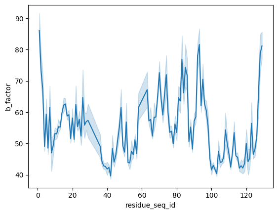
We can also easily properties such as b-factors in the TCR variable domain.

[13]:

import seaborn as sns

[14]:

tcr_variable_df = tcr_df.query('residue_seq_id <= 129')
sns.lineplot(x=tcr_variable_df['residue_seq_id'], y=tcr_variable_df['b_factor'])

[14]:

<Axes: xlabel='residue_seq_id', ylabel='b_factor'>

../_images/source_Working_with_PDB_Structures_in_Pandas_21_1.png

Computing things like contacting residues between the TCR CDR loops and the peptide is a breeze.

[15]:

import numpy as np

[16]:

CONTACT_DISTANCE = 5  # Angstroms (Å)

def euclidean_distance(x1, y1, z1, x2, y2, z2):
    return np.sqrt((x2 - x1)**2 + (y2 - y1)**2  + (z2 - z1)**2)


interface = tcr_cdrs_df.merge(peptide_df, how='cross', suffixes=('_tcr', '_peptide'))
interface['atom_distances'] = euclidean_distance(interface['pos_x_tcr'], interface['pos_y_tcr'], interface['pos_z_tcr'],
                                                 interface['pos_x_peptide'], interface['pos_y_peptide'], interface['pos_z_peptide'])

contacting_atoms = interface[interface['atom_distances'] <= CONTACT_DISTANCE]
contacting_residues = contacting_atoms[['chain_id_tcr', 'residue_seq_id_tcr', 'residue_insert_code_tcr', 'cdr', 'chain_type',
                                        'residue_seq_id_peptide', 'residue_insert_code_peptide']].drop_duplicates()

contacting_residues

[16]:

	chain_id_tcr	residue_seq_id_tcr	residue_insert_code_tcr	cdr	chain_type	residue_seq_id_peptide	residue_insert_code_peptide
6424	E	108	None	3.0	beta	8	None
6603	E	109	None	3.0	beta	9	None
6641	E	109	None	3.0	beta	7	None
6704	E	109	None	3.0	beta	8	None
6926	E	110	None	3.0	beta	7	None
7151	E	111	None	3.0	beta	7	None
7194	E	111	None	3.0	beta	4	None
7253	E	111	None	3.0	beta	5	None
7261	E	111	None	3.0	beta	6	None
7280	E	111	None	3.0	beta	8	None
7361	E	111	None	3.0	beta	3	None
7594	E	112	None	3.0	beta	4	None
7596	E	112	None	3.0	beta	5	None
7603	E	112	None	3.0	beta	6	None
7607	E	112	None	3.0	beta	7	None
7622	E	112	None	3.0	beta	8	None
8114	E	113	None	3.0	beta	5	None
11763	D	37	None	1.0	alpha	5	None
11923	D	37	None	1.0	alpha	4	None
12030	D	37	None	1.0	alpha	2	None
12033	D	37	None	1.0	alpha	3	None
12218	D	38	None	1.0	alpha	5	None
13131	D	57	None	2.0	alpha	5	None

Finally, if we want to save part of the data frame as a PDB file, we can convert it back to a Structure object and save it to a file.

[17]:

import warnings

from python_pdb.entities import Structure, StructureConstructionWarning

[18]:

# Suppressing warnings here because there are alternate locations specified in this PDB file
with warnings.catch_warnings():
    warnings.filterwarnings('ignore', category=StructureConstructionWarning)
    tcr_structure = Structure.from_pandas(tcr_df)

with open('tcr.pdb', 'w') as fh:
    fh.write(str(tcr_structure))

[19]:

!ls | grep '.pdb'

tcr.pdb

[20]:

!head tcr.pdb

ATOM     58  N   SER E   1      44.786  19.936  31.694  1.00 91.71           N
ATOM     59  CA  SER E   1      43.328  20.085  31.879  1.00 88.14           C
ATOM     60  C   SER E   1      42.582  19.234  30.860  1.00 80.31           C
ATOM     61  O   SER E   1      41.944  19.762  29.940  1.00 81.48           O
ATOM     62  CB  SER E   1      42.912  21.571  31.778  1.00 93.53           C
ATOM     63  OG  SER E   1      41.483  21.690  31.841  1.00 93.62           O
ATOM     64  N   GLN E   2      42.634  17.921  31.043  1.00 72.67           N
ATOM     65  CA  GLN E   2      41.716  17.039  30.308  1.00 69.30           C
ATOM     66  C   GLN E   2      40.246  17.307  30.674  1.00 66.83           C
ATOM     67  O   GLN E   2      39.999  17.911  31.668  1.00 70.99           O