Ascertaining the generalisability of the structure data
Introduction
In this notebook, we set out to ascertain the generalisability of our data and analysis to the broader TCR space. We compared sequence properties of our dataset to a background of TCR sequences sampled from OTS and also look at how the selected structures fit in the overall available TCR structures space.
[1]:
import matplotlib.pyplot as plt
import numpy as np
import pandas as pd
import seaborn as sns
[2]:
def rmsd(x: np.ndarray) -> float:
    '''Compute the RMSD of an array.'''
    x_bar = np.mean(x)
    n = len(x)
    return np.sqrt(np.sum((x - x_bar) ** 2) / n)
Load Data
Load OTS data
[3]:
ots_sample = pd.read_csv('../data/interim/ots_sample.csv')
ots_sample
[3]:
| cdr1_aa_alpha | cdr2_aa_alpha | cdr3_aa_alpha | cdr1_aa_beta | cdr2_aa_beta | cdr3_aa_beta | v_call_alpha | v_call_beta | j_call_alpha | j_call_beta | Species | sample_num | |
|---|---|---|---|---|---|---|---|---|---|---|---|---|
| 0 | TISGNEY | GLKNN | IVRVVWGGGADGLT | SGHDN | FVKESK | ASSLLGVSTDTQY | TRAV26-1*01 | TRBV14*01 | TRAJ45*01 | TRBJ2-3*01 | human | 1 |
| 1 | NSMFDY | ISSIKDK | AASAQGGSYIPT | LGHDT | YNNKEL | ASSRRPTDTQY | TRAV29/DV5*04 | TRBV3-1*01 | TRAJ6*01 | TRBJ2-3*01 | human | 1 |
| 2 | SSNFYA | MTLNGDE | ALGRNSGNTPLV | SGHAT | FQNNGV | ASNLAGAYEQY | TRAV24*01 | TRBV11-2*01 | TRAJ29*01 | TRBJ2-7*01 | human | 1 |
| 3 | SSVPPY | YTTGATLV | AVSEPGSQGNLI | DFQATT | SNEGSKA | SALGQPLGETQY | TRAV8-4*01 | TRBV20-1*02 | TRAJ42*01 | TRBJ2-5*01 | human | 1 |
| 4 | TSGFNG | NVLDGL | AVRDLRGSQGNLI | MGHRA | YSYEKL | ASSQAPQGADTQY | TRAV1-2*01 | TRBV4-1*01 | TRAJ42*01 | TRBJ2-3*01 | human | 1 |
| ... | ... | ... | ... | ... | ... | ... | ... | ... | ... | ... | ... | ... |
| 9995 | SSVSVY | YLSGSTLV | AVSVRGSQGNLI | MNHNY | SVGAGI | ASSYGNREGYT | TRAV8-6*01 | TRBV6-6*01 | TRAJ42*01 | TRBJ1-2*01 | human | 10 |
| 9996 | NSAFQY | TYSSGN | AMRRNTNAGKST | DFQATT | SNEGSKA | SAPTDPAGTEAF | TRAV12-3*01 | TRBV20-1*01 | TRAJ27*01 | TRBJ1-1*01 | human | 10 |
| 9997 | SVFSS | VVTGGEV | AAIIQGAQKLV | MDHEN | SYDVKM | ASSYQYYEQY | TRAV27*01 | TRBV28*01 | TRAJ54*01 | TRBJ2-7*01 | human | 10 |
| 9998 | DSAIYN | IQSSQRE | APYSGGGADGLT | SEHNR | FQNEAQ | ASSSGTGGVEHGYT | TRAV21*02 | TRBV7-9*01 | TRAJ45*01 | TRBJ1-2*01 | human | 10 |
| 9999 | NSAFQY | TYSSGN | AMTGAGSYQLT | LGHNA | YSLEER | ASSQELLGAELHYGYT | TRAV12-3*01 | TRBV4-3*01 | TRAJ28*01 | TRBJ1-2*01 | human | 10 |
10000 rows × 12 columns
[4]:
ots_sample_genes = ots_sample[['v_call_alpha', 'v_call_beta', 'j_call_alpha', 'j_call_beta', 'sample_num']].copy()

ots_sample_genes['alpha_subgroup'] = ots_sample_genes['v_call_alpha'].str.extract(r'^(TRAV\d+)')
ots_sample_genes['beta_subgroup'] = ots_sample_genes['v_call_beta'].str.extract(r'^(TRBV\d+)')

ots_sample_genes
[4]:
| v_call_alpha | v_call_beta | j_call_alpha | j_call_beta | sample_num | alpha_subgroup | beta_subgroup | |
|---|---|---|---|---|---|---|---|
| 0 | TRAV26-1*01 | TRBV14*01 | TRAJ45*01 | TRBJ2-3*01 | 1 | TRAV26 | TRBV14 |
| 1 | TRAV29/DV5*04 | TRBV3-1*01 | TRAJ6*01 | TRBJ2-3*01 | 1 | TRAV29 | TRBV3 |
| 2 | TRAV24*01 | TRBV11-2*01 | TRAJ29*01 | TRBJ2-7*01 | 1 | TRAV24 | TRBV11 |
| 3 | TRAV8-4*01 | TRBV20-1*02 | TRAJ42*01 | TRBJ2-5*01 | 1 | TRAV8 | TRBV20 |
| 4 | TRAV1-2*01 | TRBV4-1*01 | TRAJ42*01 | TRBJ2-3*01 | 1 | TRAV1 | TRBV4 |
| ... | ... | ... | ... | ... | ... | ... | ... |
| 9995 | TRAV8-6*01 | TRBV6-6*01 | TRAJ42*01 | TRBJ1-2*01 | 10 | TRAV8 | TRBV6 |
| 9996 | TRAV12-3*01 | TRBV20-1*01 | TRAJ27*01 | TRBJ1-1*01 | 10 | TRAV12 | TRBV20 |
| 9997 | TRAV27*01 | TRBV28*01 | TRAJ54*01 | TRBJ2-7*01 | 10 | TRAV27 | TRBV28 |
| 9998 | TRAV21*02 | TRBV7-9*01 | TRAJ45*01 | TRBJ1-2*01 | 10 | TRAV21 | TRBV7 |
| 9999 | TRAV12-3*01 | TRBV4-3*01 | TRAJ28*01 | TRBJ1-2*01 | 10 | TRAV12 | TRBV4 |
10000 rows × 7 columns
[5]:
ots_sample_cdrs = ots_sample.filter(regex=r'^cdr\d_aa_[alpha|beta]', axis=1)
cdr_cols = ots_sample_cdrs.columns.tolist()

ots_sample_cdrs = pd.concat([ots_sample_cdrs, ots_sample['sample_num']], axis='columns')

ots_sample_cdrs = ots_sample_cdrs.melt(id_vars='sample_num',
                                       value_vars=cdr_cols,
                                       var_name='cdr_type',
                                       value_name='sequence')
ots_sample_cdrs[['cdr', 'chain_type']] = ots_sample_cdrs['cdr_type'].str.extract('cdr(\d)_aa_(alpha|beta)')

ots_sample_cdrs['length'] = ots_sample_cdrs['sequence'].str.len()

ots_sample_cdrs
[5]:
| sample_num | cdr_type | sequence | cdr | chain_type | length | |
|---|---|---|---|---|---|---|
| 0 | 1 | cdr1_aa_alpha | TISGNEY | 1 | alpha | 7 |
| 1 | 1 | cdr1_aa_alpha | NSMFDY | 1 | alpha | 6 |
| 2 | 1 | cdr1_aa_alpha | SSNFYA | 1 | alpha | 6 |
| 3 | 1 | cdr1_aa_alpha | SSVPPY | 1 | alpha | 6 |
| 4 | 1 | cdr1_aa_alpha | TSGFNG | 1 | alpha | 6 |
| ... | ... | ... | ... | ... | ... | ... |
| 59995 | 10 | cdr3_aa_beta | ASSYGNREGYT | 3 | beta | 11 |
| 59996 | 10 | cdr3_aa_beta | SAPTDPAGTEAF | 3 | beta | 12 |
| 59997 | 10 | cdr3_aa_beta | ASSYQYYEQY | 3 | beta | 10 |
| 59998 | 10 | cdr3_aa_beta | ASSSGTGGVEHGYT | 3 | beta | 14 |
| 59999 | 10 | cdr3_aa_beta | ASSQELLGAELHYGYT | 3 | beta | 16 |
60000 rows × 6 columns
Load STCRDab data
[6]:
stcrdab_summary = pd.read_csv('../data/raw/stcrdab/db_summary.dat', delimiter='\t')
stcrdab_summary
[6]:
| pdb | Bchain | Achain | Dchain | Gchain | TCRtype | model | antigen_chain | antigen_type | antigen_name | ... | authors | resolution | method | r_free | r_factor | affinity | affinity_method | affinity_temperature | affinity_pmid | engineered | |
|---|---|---|---|---|---|---|---|---|---|---|---|---|---|---|---|---|---|---|---|---|---|
| 0 | 7zt2 | E | D | NaN | NaN | abTCR | 0 | A | A | protein | Hapten | major histocompatibility complex class i-relat... | ... | Karuppiah, V., Srikannathasan, V., Robinson, R.A. | 2.4 | X-RAY DIFFRACTION | 0.276 | 0.215 | NaN | NaN | NaN | NaN | True |
| 1 | 7zt3 | E | D | NaN | NaN | abTCR | 0 | A | protein | major histocompatibility complex class i-relat... | ... | Karuppiah, V., Srikannathasan, V., Robinson, R.A. | 2.4 | X-RAY DIFFRACTION | 0.236 | 0.191 | NaN | NaN | NaN | NaN | True |
| 2 | 7zt4 | E | D | NaN | NaN | abTCR | 0 | A | protein | major histocompatibility complex class i-relat... | ... | Karuppiah, V., Robinson, R.A. | 2.02 | X-RAY DIFFRACTION | 0.268 | 0.234 | NaN | NaN | NaN | NaN | True |
| 3 | 7zt5 | E | D | NaN | NaN | abTCR | 0 | A | protein | major histocompatibility complex class i-relat... | ... | Karuppiah, V., Robinson, R.A. | 2.09 | X-RAY DIFFRACTION | 0.266 | 0.225 | NaN | NaN | NaN | NaN | True |
| 4 | 7zt7 | E | D | NaN | NaN | abTCR | 0 | A | protein | major histocompatibility complex class i-relat... | ... | Karuppiah, V., Robinson, R.A. | 1.84 | X-RAY DIFFRACTION | 0.255 | 0.207 | NaN | NaN | NaN | NaN | True |
| ... | ... | ... | ... | ... | ... | ... | ... | ... | ... | ... | ... | ... | ... | ... | ... | ... | ... | ... | ... | ... | ... |
| 931 | 3rtq | D | C | NaN | NaN | abTCR | 0 | A | Hapten | N-[(2S,3S,4R)-3,4-DIHYDROXY-1-{[(1S,2S,3R,4R,5... | ... | Yu, E.D., Zajonc, D.M. | 2.8 | X-RAY DIFFRACTION | 0.268 | 0.227 | NaN | NaN | NaN | NaN | True |
| 932 | 3dxa | O | N | NaN | NaN | abTCR | 0 | M | peptide | ebv decapeptide epitope | ... | Archbold, J.K., Macdonald, W.A., Gras, S., Ros... | 3.5 | X-RAY DIFFRACTION | 0.330 | 0.286 | NaN | NaN | NaN | NaN | True |
| 933 | 1d9k | B | A | NaN | NaN | abTCR | 0 | P | peptide | conalbumin peptide | ... | Reinherz, E.L., Tan, K., Tang, L., Kern, P., L... | 3.2 | X-RAY DIFFRACTION | 0.293 | 0.247 | NaN | NaN | NaN | NaN | True |
| 934 | 4gg6 | H | G | NaN | NaN | abTCR | 0 | J | peptide | peptide from alpha/beta-gliadin mm1 | ... | Broughton, S.E., Theodossis, A., Petersen, J.,... | 3.2 | X-RAY DIFFRACTION | 0.285 | 0.246 | NaN | NaN | NaN | NaN | True |
| 935 | 2apf | A | NaN | NaN | NaN | NaN | 0 | NaN | NaN | NaN | ... | Cho, S., Swaminathan, C.P., Yang, J., Kerzic, ... | 1.8 | X-RAY DIFFRACTION | 0.263 | 0.197 | NaN | NaN | NaN | NaN | True |
936 rows × 39 columns
Load apo-holo data
[7]:
apo_holo_summary = pd.read_csv('../data/processed/apo-holo-tcr-pmhc-class-I/apo_holo_summary.csv')
apo_holo_summary
[7]:
| file_name | pdb_id | structure_type | state | alpha_chain | beta_chain | antigen_chain | mhc_chain1 | mhc_chain2 | cdr_sequences_collated | peptide_sequence | mhc_slug | |
|---|---|---|---|---|---|---|---|---|---|---|---|---|
| 0 | 1ao7_D-E-C-A-B_tcr_pmhc.pdb | 1ao7 | tcr_pmhc | holo | D | E | C | A | B | DRGSQS-IYSNGD-AVTTDSWGKLQ-MNHEY-SVGAGI-ASRPGLA... | LLFGYPVYV | hla_a_02_01 |
| 1 | 1b0g_C-A-B_pmhc.pdb | 1b0g | pmhc | apo | NaN | NaN | C | A | B | NaN | ALWGFFPVL | hla_a_02_01 |
| 2 | 1b0g_F-D-E_pmhc.pdb | 1b0g | pmhc | apo | NaN | NaN | F | D | E | NaN | ALWGFFPVL | hla_a_02_01 |
| 3 | 1bd2_D-E-C-A-B_tcr_pmhc.pdb | 1bd2 | tcr_pmhc | holo | D | E | C | A | B | NSMFDY-ISSIKDK-AAMEGAQKLV-MNHEY-SVGAGI-ASSYPGG... | LLFGYPVYV | hla_a_02_01 |
| 4 | 1bii_P-A-B_pmhc.pdb | 1bii | pmhc | apo | NaN | NaN | P | A | B | NaN | RGPGRAFVTI | h2_dd |
| ... | ... | ... | ... | ... | ... | ... | ... | ... | ... | ... | ... | ... |
| 386 | 7rtd_C-A-B_pmhc.pdb | 7rtd | pmhc | apo | NaN | NaN | C | A | B | NaN | YLQPRTFLL | hla_a_02_01 |
| 387 | 7rtr_D-E-C-A-B_tcr_pmhc.pdb | 7rtr | tcr_pmhc | holo | D | E | C | A | B | DRGSQS-IYSNGD-AVNRDDKII-SEHNR-FQNEAQ-ASSPDIEQY | YLQPRTFLL | hla_a_02_01 |
| 388 | 8gvb_A-B-P-H-L_tcr_pmhc.pdb | 8gvb | tcr_pmhc | holo | A | B | P | H | L | YGATPY-YFSGDTLV-AVGFTGGGNKLT-SEHNR-FQNEAQ-ASSD... | RYPLTFGW | hla_a_24_02 |
| 389 | 8gvg_A-B-P-H-L_tcr_pmhc.pdb | 8gvg | tcr_pmhc | holo | A | B | P | H | L | YGATPY-YFSGDTLV-AVGFTGGGNKLT-SEHNR-FQNEAQ-ASSD... | RFPLTFGW | hla_a_24_02 |
| 390 | 8gvi_A-B-P-H-L_tcr_pmhc.pdb | 8gvi | tcr_pmhc | holo | A | B | P | H | L | YGATPY-YFSGDTLV-AVVFTGGGNKLT-SEHNR-FQNEAQ-ASSL... | RYPLTFGW | hla_a_24_02 |
391 rows × 12 columns
[8]:
apo_holo_genes = apo_holo_summary.copy().merge(
    stcrdab_summary,
    how='left',
    left_on=['pdb_id', 'alpha_chain', 'beta_chain'],
    right_on=['pdb', 'Achain', 'Bchain'],
).drop_duplicates(['cdr_sequences_collated'])[['alpha_subgroup', 'beta_subgroup']]
[9]:
apo_holo_cdr_sequences = apo_holo_summary['cdr_sequences_collated'].str.split('-').apply(pd.Series)
apo_holo_cdr_sequences.columns = ['cdr1_alpha', 'cdr2_alpha', 'cdr3_alpha', 'cdr1_beta', 'cdr2_beta', 'cdr3_beta']

apo_holo_cdr_sequences = apo_holo_cdr_sequences.drop_duplicates()
apo_holo_cdr_sequences = apo_holo_cdr_sequences.dropna()

apo_holo_cdr_sequences
apo_holo_cdr_sequences = apo_holo_cdr_sequences.melt(value_vars=apo_holo_cdr_sequences.columns,
                                                     var_name='cdr_type',
                                                     value_name='sequence')
apo_holo_cdr_sequences[['cdr', 'chain_type']] = apo_holo_cdr_sequences['cdr_type'].str.extract('cdr(\d)_(alpha|beta)')

apo_holo_cdr_sequences['length'] = apo_holo_cdr_sequences['sequence'].str.len()

apo_holo_cdr_sequences
[9]:
| cdr_type | sequence | cdr | chain_type | length | |
|---|---|---|---|---|---|
| 0 | cdr1_alpha | DRGSQS | 1 | alpha | 6 |
| 1 | cdr1_alpha | NSMFDY | 1 | alpha | 6 |
| 2 | cdr1_alpha | TQDSSYF | 1 | alpha | 7 |
| 3 | cdr1_alpha | YSATPY | 1 | alpha | 6 |
| 4 | cdr1_alpha | TISGTDY | 1 | alpha | 7 |
| ... | ... | ... | ... | ... | ... |
| 511 | cdr3_beta | ASSSANSGELF | 3 | beta | 11 |
| 512 | cdr3_beta | ASSYGTGINYGYT | 3 | beta | 13 |
| 513 | cdr3_beta | ASSLDPGDTGELF | 3 | beta | 13 |
| 514 | cdr3_beta | ASSDRDRVPETQY | 3 | beta | 13 |
| 515 | cdr3_beta | ASSLRDRVPETQY | 3 | beta | 13 |
516 rows × 5 columns
Compare CDR Lengths
[10]:
ots_sample_cdrs['source'] = 'OTS'
apo_holo_cdr_sequences['source'] = 'STCRDab'

cdr_lengths = pd.concat([ots_sample_cdrs, apo_holo_cdr_sequences])
cdr_lengths
[10]:
| sample_num | cdr_type | sequence | cdr | chain_type | length | source | |
|---|---|---|---|---|---|---|---|
| 0 | 1.0 | cdr1_aa_alpha | TISGNEY | 1 | alpha | 7 | OTS |
| 1 | 1.0 | cdr1_aa_alpha | NSMFDY | 1 | alpha | 6 | OTS |
| 2 | 1.0 | cdr1_aa_alpha | SSNFYA | 1 | alpha | 6 | OTS |
| 3 | 1.0 | cdr1_aa_alpha | SSVPPY | 1 | alpha | 6 | OTS |
| 4 | 1.0 | cdr1_aa_alpha | TSGFNG | 1 | alpha | 6 | OTS |
| ... | ... | ... | ... | ... | ... | ... | ... |
| 511 | NaN | cdr3_beta | ASSSANSGELF | 3 | beta | 11 | STCRDab |
| 512 | NaN | cdr3_beta | ASSYGTGINYGYT | 3 | beta | 13 | STCRDab |
| 513 | NaN | cdr3_beta | ASSLDPGDTGELF | 3 | beta | 13 | STCRDab |
| 514 | NaN | cdr3_beta | ASSDRDRVPETQY | 3 | beta | 13 | STCRDab |
| 515 | NaN | cdr3_beta | ASSLRDRVPETQY | 3 | beta | 13 | STCRDab |
60516 rows × 7 columns
[11]:
ots_sample_cdrs_proptions = (ots_sample_cdrs.groupby(['chain_type', 'cdr', 'sample_num'])
                                            ['length']
                                            .value_counts(normalize=True)
                                            * 100)
ots_sample_cdrs_proptions.name = 'percentage'
ots_sample_cdrs_proptions = ots_sample_cdrs_proptions.reset_index()
[12]:
ots_sample_cdrs_proptions_agg = (ots_sample_cdrs_proptions.groupby(['chain_type', 'cdr', 'length'])
                                                          .agg({'percentage': ['mean', 'sem']})
                                                          .fillna(0.0)
                                                          .reset_index())
ots_sample_cdrs_proptions_agg.columns = ['_'.join(col).rstrip('_').replace('_mean', '')
                                         for col in ots_sample_cdrs_proptions_agg.columns]
[13]:
apo_holo_cdr_length_proportions = (apo_holo_cdr_sequences.groupby(['chain_type', 'cdr'])
                                   ['length']
                                   .value_counts(normalize=True)
                                   * 100)
apo_holo_cdr_length_proportions.name = 'percentage'
apo_holo_cdr_length_proportions = apo_holo_cdr_length_proportions.reset_index()
[14]:
cdr_length_proportions = ots_sample_cdrs_proptions_agg.merge(apo_holo_cdr_length_proportions,
                                                             how='outer',
                                                             on=['chain_type', 'cdr', 'length'],
                                                             suffixes=['_ots', '_stcrdab']).fillna(0)


cdr_length_proportions['difference'] = (cdr_length_proportions['percentage_stcrdab']
                                        - cdr_length_proportions['percentage_ots'])
[15]:
cdr_length_percentages = (cdr_lengths.groupby(['chain_type', 'cdr', 'sample_num', 'source'], dropna=False)
                                     ['length']
                                     .value_counts(normalize=True)
                                     * 100)
cdr_length_percentages.name = 'percentage'
cdr_length_percentages = cdr_length_percentages.reset_index()
[16]:
for (chain_type, cdr), group in cdr_length_percentages.groupby(['chain_type', 'cdr']):
    length_min = group['length'].min()
    length_max = group['length'].max()
    expected_length_values = set(range(length_min, length_max + 1))

    actual_length_values = set(group['length'].unique())
    missing_length_values = expected_length_values - actual_length_values
    missing_length_values = sorted(list(missing_length_values))

    if len(missing_length_values) > 0:
        missing_entries = pd.DataFrame({'chain_type': [chain_type for _ in missing_length_values],
                                        'cdr': [cdr for _ in missing_length_values],
                                        'source': ['OTS' for _ in missing_length_values],
                                        'length': missing_length_values,
                                        'percentage': [0.0 for _ in missing_length_values]})

        cdr_length_percentages = pd.concat([cdr_length_percentages, missing_entries])

cdr_length_percentages = cdr_length_percentages.reset_index(drop=True)
[17]:
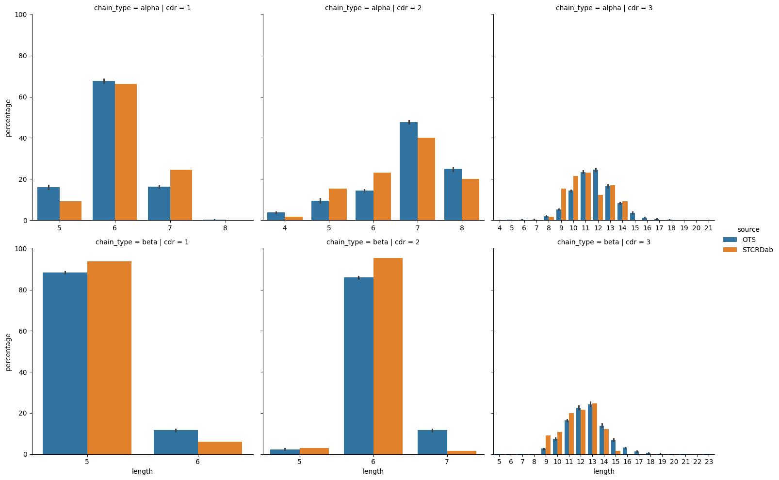
grid = sns.catplot(cdr_length_percentages,
            x='length',
            y='percentage',
            hue='source',
            row='chain_type', col='cdr',
            kind='bar', sharex=False)

plt.show()
[18]:
cdr_lengths.groupby(['chain_type', 'cdr', 'source'])['length'].agg([pd.Series.mode, 'mean', 'std'])
[18]:
| mode | mean | std | |||
|---|---|---|---|---|---|
| chain_type | cdr | source | |||
| alpha | 1 | OTS | 6 | 6.003800 | 0.570279 |
| STCRDab | 6 | 6.127907 | 0.609658 | ||
| 2 | OTS | 7 | 6.805900 | 1.031664 | |
| STCRDab | 7 | 6.546512 | 1.001845 | ||
| 3 | OTS | 12 | 11.730200 | 1.692954 | |
| STCRDab | 11 | 11.255814 | 1.688620 | ||
| beta | 1 | OTS | 5 | 5.116500 | 0.320840 |
| STCRDab | 5 | 5.069767 | 0.256249 | ||
| 2 | OTS | 6 | 6.092400 | 0.363147 | |
| STCRDab | 6 | 5.976744 | 0.215666 | ||
| 3 | OTS | 13 | 12.568400 | 1.753918 | |
| STCRDab | 12 | 12.046512 | 1.578584 |
[19]:
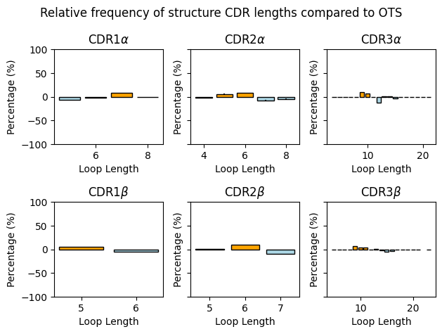
fig, axes = plt.subplots(ncols=3, nrows=2, tight_layout=True, sharey=True)
plt.ylim([-100, 100])
fig.suptitle('Relative frequency of structure CDR lengths compared to OTS')

for i, chain_type in enumerate(('alpha', 'beta')):
    for j, cdr in enumerate(('1', '2', '3')):
        proportion_data = cdr_length_proportions.query("chain_type == @chain_type and cdr == @cdr")
        colors = proportion_data['difference'].map(lambda diff: 'lightblue' if diff < 0 else 'orange')

        axes[i, j].bar(proportion_data['length'], proportion_data['difference'],
                       yerr=proportion_data['percentage_sem'],
                       color=colors, edgecolor='black')

        axes[i, j].set_title(f'CDR{cdr}$\\{chain_type}$')
        axes[i, j].set_xlabel('Loop Length')
        axes[i, j].set_ylabel('Percentage (%)')

plt.show()
[20]:
for chain_type in ('alpha', 'beta'):
    for cdr in ('1', '2', '3'):
        proportion_data = cdr_length_proportions.query("chain_type == @chain_type and cdr == @cdr")
        print(f'CDR{cdr}{chain_type} RMSD:', round(rmsd(proportion_data['difference']), 2))

print()
print('Overall RMSD:', round(rmsd(cdr_length_proportions['difference']), 2))
CDR1alpha RMSD: 5.8
CDR2alpha RMSD: 7.14
CDR3alpha RMSD: 4.41
CDR1beta RMSD: 4.67
CDR2beta RMSD: 8.15
CDR3beta RMSD: 2.36

Overall RMSD: 4.65
Overall, it seems that the distribution of lengths is similar between the apo-holo structures taken from the STCRDab and the background TCRs from OTS. The distributions look similar between the data sources, with a slightly larger variety for the OTS TCRs. Also, the mode length for each CDR type is the same between the OTS background and the dataset used in this analysis (6 for CDR1α, 7 for CDR2α, 11 for CDR3α, 5 for CDR1β, 6 for CDR2β, and 13 for CDR3β).
Compare TCR V Gene Usage
[21]:
ots_sample_genes['source'] = 'OTS'
apo_holo_genes['source'] = 'STCRDab'

gene_usage = pd.concat([ots_sample_genes, apo_holo_genes])
gene_usage = gene_usage.dropna(subset=['alpha_subgroup', 'beta_subgroup'])
gene_usage = gene_usage.melt(id_vars=['sample_num', 'source'],
                             value_vars=['alpha_subgroup', 'beta_subgroup'],
                             var_name='subgroup', value_name='gene')

gene_usage['subgroup_num'] = gene_usage['gene'].str.extract(r'TR[A|B]V(\d+)', expand=False).apply(int)

gene_usage
[21]:
| sample_num | source | subgroup | gene | subgroup_num | |
|---|---|---|---|---|---|
| 0 | 1.0 | OTS | alpha_subgroup | TRAV26 | 26 |
| 1 | 1.0 | OTS | alpha_subgroup | TRAV29 | 29 |
| 2 | 1.0 | OTS | alpha_subgroup | TRAV24 | 24 |
| 3 | 1.0 | OTS | alpha_subgroup | TRAV8 | 8 |
| 4 | 1.0 | OTS | alpha_subgroup | TRAV1 | 1 |
| ... | ... | ... | ... | ... | ... |
| 20163 | NaN | STCRDab | beta_subgroup | TRBV7 | 7 |
| 20164 | NaN | STCRDab | beta_subgroup | TRBV6 | 6 |
| 20165 | NaN | STCRDab | beta_subgroup | TRBV11 | 11 |
| 20166 | NaN | STCRDab | beta_subgroup | TRBV7 | 7 |
| 20167 | NaN | STCRDab | beta_subgroup | TRBV7 | 7 |
20168 rows × 5 columns
[22]:
gene_usage_percentages = (gene_usage.groupby(['subgroup', 'source', 'sample_num'], dropna=False)
                                    [['gene', 'subgroup_num']]
                                    .value_counts(normalize=True)
                                    * 100)
gene_usage_percentages.name = 'percentage'

gene_usage_percentages = gene_usage_percentages.reset_index()
[23]:
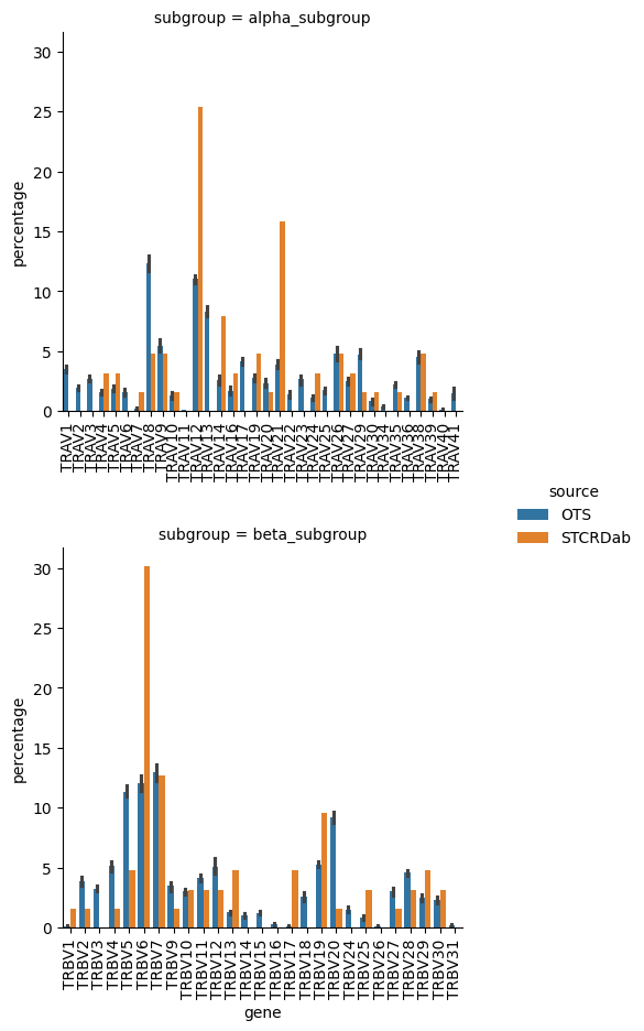
grid = sns.catplot(gene_usage_percentages.sort_values(['subgroup', 'subgroup_num']),
            row='subgroup',
            x='gene', y='percentage',
            hue='source',
            kind='bar',
            sharex=False)

for ax in grid.axes.flat:
    ax.set_xticklabels(ax.get_xticklabels(), rotation=90)

grid.tight_layout(pad=3.0)

plt.show()
/var/scratch/bmcmaste/2178229/ipykernel_2150264/1817500796.py:9: UserWarning: FixedFormatter should only be used together with FixedLocator
  ax.set_xticklabels(ax.get_xticklabels(), rotation=90)
[24]:
ots_sample_gene_usage_percentages = gene_usage_percentages.query("source == 'OTS'")
ots_sample_gene_usage_percentages_agg = (ots_sample_gene_usage_percentages.groupby(['gene', 'subgroup', 'subgroup_num'])
                                                                          .agg({'percentage': ['mean', 'sem']})
                                                                          .reset_index()
                                                                          .fillna(0.0))

ots_sample_gene_usage_percentages_agg.columns = ['_'.join(col).rstrip('_').replace('_mean', '')
                                                 for col in ots_sample_gene_usage_percentages_agg.columns]
[25]:
apo_holo_gene_usage_percentages = gene_usage_percentages.query("source == 'STCRDab'")
gene_usage_percentages_compare = apo_holo_gene_usage_percentages.merge(ots_sample_gene_usage_percentages_agg,
                                                                       how='outer',
                                                                       on=['gene', 'subgroup', 'subgroup_num'],
                                                                       suffixes=('_stcrdab', '_ots'))

gene_usage_percentages_compare = gene_usage_percentages_compare.drop(['source', 'sample_num'], axis='columns')
gene_usage_percentages_compare = gene_usage_percentages_compare.fillna(0.0)

gene_usage_percentages_compare['difference'] = (gene_usage_percentages_compare['percentage_stcrdab']
                                                - gene_usage_percentages_compare['percentage_ots'])
[26]:
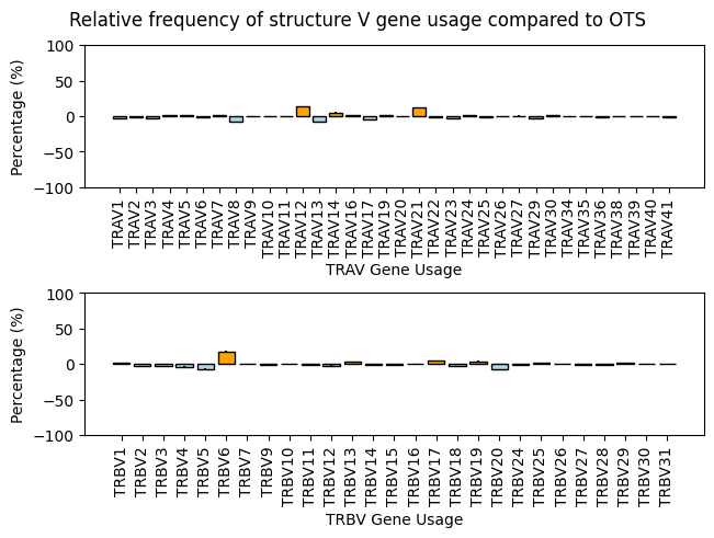
fig, axes = plt.subplots(nrows=2, constrained_layout=True, sharey=True)
plt.ylim([-100, 100])
fig.suptitle('Relative frequency of structure V gene usage compared to OTS')

for i, subgroup in enumerate(('alpha_subgroup', 'beta_subgroup')):
    plot_data = gene_usage_percentages_compare.query('subgroup == @subgroup').sort_values('subgroup_num')

    colors = plot_data['difference'].map(lambda diff: 'lightblue' if diff < 0 else 'orange')

    axes[i].bar(plot_data['gene'],
               plot_data['difference'],
               yerr=plot_data['percentage_sem'],
               color=colors,
               edgecolor='black')

    axes[i].set_xlabel(f"TR{'A' if subgroup == 'alpha_subgroup' else 'B'}V Gene Usage")
    axes[i].set_ylabel('Percentage (%)')
    axes[i].tick_params(axis='x', labelrotation=90)

plt.show()
[27]:
print('TRAV Gene Usage RMSD:',
      round(rmsd(gene_usage_percentages_compare.query("subgroup == 'alpha_subgroup'")['difference']), 2))

print('TRBV Gene Usage RMSD:',
      round(rmsd(gene_usage_percentages_compare.query("subgroup == 'beta_subgroup'")['difference']), 2))
TRAV Gene Usage RMSD: 4.33
TRBV Gene Usage RMSD: 4.24
The gene usage between apo-holo TCRs from STCRDab and the background TCRs from OTS is largely similar. There are a few exceptions in the STCRDab structures that show an over-representation of certain gene usages. For exampe, TRAV12, TRAV14, TRAV21, and TRBV6 all seem to be in higher abundance in the STCRDab data compared with the OTS background.
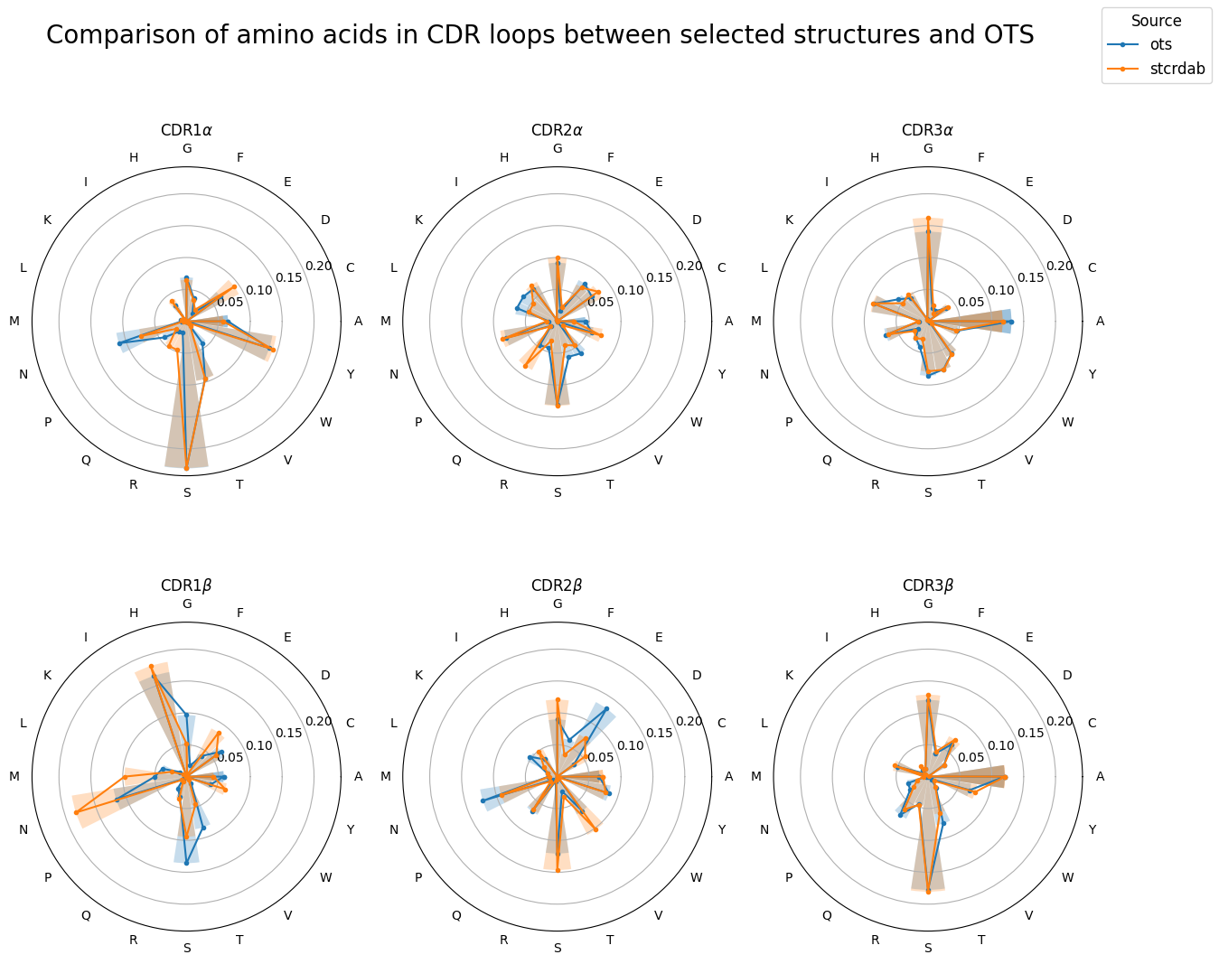
Comparison of amino acide types in loops
[28]:
AMINO_ACIDS = ['A', 'C', 'D', 'E', 'F', 'G', 'H', 'I', 'K', 'L', 'M', 'N', 'P', 'Q', 'R', 'S', 'T', 'V', 'W', 'Y']

def count_amino_acids(residues: pd.Series, normalize = True) -> pd.Series:
    counts = {res: 0 for res in AMINO_ACIDS}

    for res in residues.tolist():
        counts[res] += 1

    if normalize:
        num_residues = len(residues)
        counts = {res: count / num_residues for res, count in counts.items()}

    counts = pd.Series(counts)
    counts.name = 'count' if not normalize else 'proportion'
    counts.index.name = 'residue'

    return counts
[29]:
ots_sample_cdrs_residues = ots_sample_cdrs[['sample_num', 'chain_type', 'cdr', 'sequence']].copy()
ots_sample_cdrs_residues['residue'] = ots_sample_cdrs_residues['sequence'].map(list)
ots_sample_cdrs_residues = ots_sample_cdrs_residues.explode('residue')

ots_sample_cdrs_residues_counts = (ots_sample_cdrs_residues.groupby(['sample_num', 'chain_type', 'cdr'])
                                                            ['residue']
                                                            .apply(count_amino_acids))
ots_sample_cdrs_residues_counts.name = 'proportion'
ots_sample_cdrs_residues_counts = ots_sample_cdrs_residues_counts.to_frame()
ots_sample_cdrs_residues_counts = ots_sample_cdrs_residues_counts.reset_index()

ots_sample_cdrs_residues_counts
[29]:
| sample_num | chain_type | cdr | residue | proportion | |
|---|---|---|---|---|---|
| 0 | 1 | alpha | 1 | A | 0.067791 |
| 1 | 1 | alpha | 1 | C | 0.000000 |
| 2 | 1 | alpha | 1 | D | 0.062615 |
| 3 | 1 | alpha | 1 | E | 0.014527 |
| 4 | 1 | alpha | 1 | F | 0.033228 |
| ... | ... | ... | ... | ... | ... |
| 1195 | 10 | beta | 3 | S | 0.181695 |
| 1196 | 10 | beta | 3 | T | 0.073013 |
| 1197 | 10 | beta | 3 | V | 0.021305 |
| 1198 | 10 | beta | 3 | W | 0.006623 |
| 1199 | 10 | beta | 3 | Y | 0.066949 |
1200 rows × 5 columns
[30]:
ots_sample_cdrs_residues_counts_agg = (ots_sample_cdrs_residues_counts.groupby(['chain_type', 'cdr', 'residue'])
                                                                      .agg({'proportion': ['mean', 'sem']})
                                                                      .reset_index())

ots_sample_cdrs_residues_counts_agg.columns = ['_'.join(col).rstrip('_').replace('_mean', '')
                                               for col in ots_sample_cdrs_residues_counts_agg.columns]
[31]:
apo_holo_cdr_sequences_residues = apo_holo_cdr_sequences[['chain_type', 'cdr', 'sequence']].copy()
apo_holo_cdr_sequences_residues['residue'] = apo_holo_cdr_sequences_residues['sequence'].map(list)
apo_holo_cdr_sequences_residues = apo_holo_cdr_sequences_residues.explode('residue')

apo_holo_cdr_sequences_residues_counts = (apo_holo_cdr_sequences_residues.groupby(['chain_type', 'cdr'])
                                          ['residue']
                                          .apply(count_amino_acids))

apo_holo_cdr_sequences_residues_counts.name = 'proportion'
apo_holo_cdr_sequences_residues_counts = apo_holo_cdr_sequences_residues_counts.to_frame()
apo_holo_cdr_sequences_residues_counts = apo_holo_cdr_sequences_residues_counts.reset_index()

apo_holo_cdr_sequences_residues_counts
[31]:
| chain_type | cdr | residue | proportion | |
|---|---|---|---|---|
| 0 | alpha | 1 | A | 0.055028 |
| 1 | alpha | 1 | C | 0.000000 |
| 2 | alpha | 1 | D | 0.087287 |
| 3 | alpha | 1 | E | 0.017078 |
| 4 | alpha | 1 | F | 0.037951 |
| ... | ... | ... | ... | ... |
| 115 | beta | 3 | S | 0.179537 |
| 116 | beta | 3 | T | 0.062741 |
| 117 | beta | 3 | V | 0.023166 |
| 118 | beta | 3 | W | 0.013514 |
| 119 | beta | 3 | Y | 0.076255 |
120 rows × 4 columns
[32]:
ots_sample_cdrs_residues_counts_agg['source'] = 'ots'
apo_holo_cdr_sequences_residues_counts['source'] = 'stcrdab'

cdr_residue_counts = pd.concat([ots_sample_cdrs_residues_counts_agg, apo_holo_cdr_sequences_residues_counts])
[33]:
angles = np.linspace(0, 2 * np.pi, len(AMINO_ACIDS), endpoint=False).tolist()
amino_acid_angles = dict(zip(AMINO_ACIDS, angles))
[34]:
fig, axes = plt.subplots(nrows=2, ncols=3,
                         figsize=(15, 12),
                         sharey=True,
                         subplot_kw={'projection': 'polar'})

lines = []
for i, chain_type in enumerate(('alpha', 'beta')):
    for j, cdr in enumerate(('1', '2', '3')):
        for source in 'ots', 'stcrdab':
            residue_counts = cdr_residue_counts[(cdr_residue_counts['source'] == source)
                                                & (cdr_residue_counts['chain_type'] == chain_type)
                                                & (cdr_residue_counts['cdr'] == cdr)].sort_values('residue')

            proportions = residue_counts['proportion'].tolist()
            label_angles = residue_counts['residue'].map(amino_acid_angles).tolist()

            # Join ends
            proportions.append(proportions[0])
            label_angles.append(label_angles[0])

            line, = axes[i, j].plot(label_angles, proportions, marker='o', markersize=3, label=source)
            axes[i, j].bar(label_angles, proportions, alpha=0.25, width=0.3)

            lines.append(line)

        axes[i, j].set_xticks(angles)
        axes[i, j].set_xticklabels(AMINO_ACIDS)
        axes[i, j].grid(which='major', axis='x', visible=False)

        axes[i, j].set_title(f'CDR{cdr}$\\{chain_type}$')

unique_handles_labels = {}
for line in lines:
    label = line.get_label()
    if label not in unique_handles_labels:
        unique_handles_labels[label] = line

labels, handles = zip(*unique_handles_labels.items())

legend = fig.legend(handles, labels, title='Source', fontsize='large')
legend.get_title().set_fontsize('large')

fig.suptitle('Comparison of amino acids in CDR loops between selected structures and OTS',
             fontsize=20)

plt.show()
[35]:
cdr_residue_counts_compare = cdr_residue_counts.pivot(index=['chain_type', 'cdr', 'residue'],
                                                      columns='source',
                                                      values='proportion').reset_index()

cdr_residue_counts_compare['difference'] = cdr_residue_counts_compare['stcrdab'] - cdr_residue_counts_compare['ots']

print(cdr_residue_counts_compare.groupby(['chain_type', 'cdr'])['difference'].agg(rmsd))

print(f"Overall RMSD: {rmsd(cdr_residue_counts_compare['difference']):.2e}")
chain_type  cdr
alpha       1      0.015719
            2      0.013582
            3      0.007108
beta        1      0.025485
            2      0.022489
            3      0.007593
Name: difference, dtype: float64
Overall RMSD: 1.68e-02
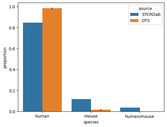
Comparison of species
[36]:
ots_organism_counts = ots_sample.groupby('sample_num')['Species'].value_counts(normalize=True)
ots_organism_counts.name = 'proportion'
ots_organism_counts = ots_organism_counts.to_frame().reset_index()
ots_organism_counts = ots_organism_counts.rename({'Species': 'species'}, axis='columns')
ots_organism_counts
[36]:
| sample_num | species | proportion | |
|---|---|---|---|
| 0 | 1 | human | 0.993 |
| 1 | 1 | mouse | 0.007 |
| 2 | 2 | human | 0.983 |
| 3 | 2 | mouse | 0.017 |
| 4 | 3 | human | 0.979 |
| 5 | 3 | mouse | 0.021 |
| 6 | 4 | human | 0.982 |
| 7 | 4 | mouse | 0.018 |
| 8 | 5 | human | 0.981 |
| 9 | 5 | mouse | 0.019 |
| 10 | 6 | human | 0.985 |
| 11 | 6 | mouse | 0.015 |
| 12 | 7 | human | 0.984 |
| 13 | 7 | mouse | 0.016 |
| 14 | 8 | human | 0.975 |
| 15 | 8 | mouse | 0.025 |
| 16 | 9 | human | 0.991 |
| 17 | 9 | mouse | 0.009 |
| 18 | 10 | human | 0.986 |
| 19 | 10 | mouse | 0.014 |
[37]:
apo_holo_annotated = apo_holo_summary.merge(
    stcrdab_summary,
    how='left',
    left_on=['pdb_id', 'alpha_chain', 'beta_chain', 'antigen_chain', 'mhc_chain1', 'mhc_chain2'],
    right_on=['pdb', 'Achain', 'Bchain', 'antigen_chain', 'mhc_chain1', 'mhc_chain2'],
)
[38]:
apo_holo_organisms = apo_holo_annotated.drop_duplicates(['cdr_sequences_collated'])[['alpha_organism', 'beta_organism']]
[39]:
apo_holo_organisms[apo_holo_organisms['alpha_organism'].notnull()
                   | apo_holo_organisms['beta_organism'].notnull()].query("alpha_organism != beta_organism")
[39]:
| alpha_organism | beta_organism |
|---|
[40]:
apo_holo_organisms = apo_holo_organisms['beta_organism']
apo_holo_organisms.unique()
[40]:
array(['homo sapiens', nan, 'mus musculus', 'mus musculus, homo sapiens'],
      dtype=object)
[41]:
apo_holo_organisms = apo_holo_organisms.map({'homo sapiens': 'human',
                                             'mus musculus': 'mouse',
                                             'mus musculus, homo sapiens': 'human/mouse'})
[42]:
apo_holo_organisms.value_counts()
[42]:
human          72
mouse          10
human/mouse     3
Name: beta_organism, dtype: int64
[43]:
apo_holo_organisms_counts = apo_holo_organisms.value_counts(normalize=True)
apo_holo_organisms_counts.name = 'proportion'
apo_holo_organisms_counts
[43]:
human          0.847059
mouse          0.117647
human/mouse    0.035294
Name: proportion, dtype: float64
[44]:
apo_holo_organisms_counts = apo_holo_organisms_counts.to_frame().reset_index(names='species')
apo_holo_organisms_counts['source'] = 'STCRDab'
apo_holo_organisms_counts['sample_num'] = 1

ots_organism_counts = ots_organism_counts
ots_organism_counts['source'] = 'OTS'

organism_counts = pd.concat([apo_holo_organisms_counts, ots_organism_counts]).reset_index(drop=True)
[45]:
sns.barplot(organism_counts, x='species', y='proportion', hue='source')
[45]:
<AxesSubplot: xlabel='species', ylabel='proportion'>
Selected structures coverage of canonical classes
[46]:
cdr_clusters = pd.read_csv('../data/processed/stcrdab_clusters.csv')
cdr_clusters
[46]:
| name | cluster | chain_type | cdr | sequence | cluster_type | |
|---|---|---|---|---|---|---|
| 0 | 7zt2_DE | 12 | alpha_chain | 1 | TSGFNG | pseudo |
| 1 | 7zt3_DE | 12 | alpha_chain | 1 | TSGFNG | pseudo |
| 2 | 7zt4_DE | 12 | alpha_chain | 1 | TSGFNG | pseudo |
| 3 | 7zt5_DE | 12 | alpha_chain | 1 | TSGFNG | pseudo |
| 4 | 7zt7_DE | 12 | alpha_chain | 1 | TSGFNG | pseudo |
| ... | ... | ... | ... | ... | ... | ... |
| 4807 | 6miv_CD | 22 | beta_chain | 3 | ASGDEGYTQY | canonical |
| 4808 | 3rtq_CD | 22 | beta_chain | 3 | ASGDEGYTQY | canonical |
| 4809 | 3dxa_NO | noise | beta_chain | 3 | ASRYRDDSYNEQF | NaN |
| 4810 | 1d9k_AB | noise | beta_chain | 3 | ASGGQGRAEQF | NaN |
| 4811 | 4gg6_GH | noise | beta_chain | 3 | ASSVAVSAGTYEQY | NaN |
4812 rows × 6 columns
[47]:
cdr_clusters[['pdb_id', 'chains']] = cdr_clusters['name'].str.split('_').apply(pd.Series)
cdr_clusters[['alpha_chain', 'beta_chain']] = cdr_clusters['chains'].apply(list).apply(pd.Series)
[48]:
common_columns = ['pdb_id', 'alpha_chain', 'beta_chain']
apo_holo_index = pd.MultiIndex.from_frame(apo_holo_summary[common_columns])

cdr_clusters['in_apo_holo'] = cdr_clusters[common_columns].apply(tuple, axis=1).isin(apo_holo_index)
[49]:
canonical_cdr_clusters = cdr_clusters.query("cluster_type == 'canonical'").copy().reset_index(drop=True)
canonical_cdr_clusters['cluster_num'] = canonical_cdr_clusters['cluster'].map(int)
[50]:
grouped = (canonical_cdr_clusters.groupby(['chain_type', 'cdr', 'cluster', 'in_apo_holo'])
                                 .size()
                                 .reset_index(name='count'))
total_counts = (canonical_cdr_clusters.groupby(['chain_type', 'cdr'])
                                      .size()
                                      .reset_index(name='total_count'))

grouped = grouped.merge(total_counts, on=['chain_type', 'cdr'])
grouped['percent'] = grouped['count'] / grouped['total_count'] * 100
[51]:
grouped['cluster_num'] = grouped['cluster'].apply(int)
grouped = grouped.sort_values('cluster_num')
[52]:
grid = sns.displot(grouped,
                   row='chain_type', col='cdr',
                   x='cluster',
                   weights='percent',
                   hue='in_apo_holo', multiple='stack',
                   facet_kws=dict(sharex=False))

grid.set_axis_labels("Cluster", "Percentage (%)")
grid.set(ylim=(0, 100))

plt.show()
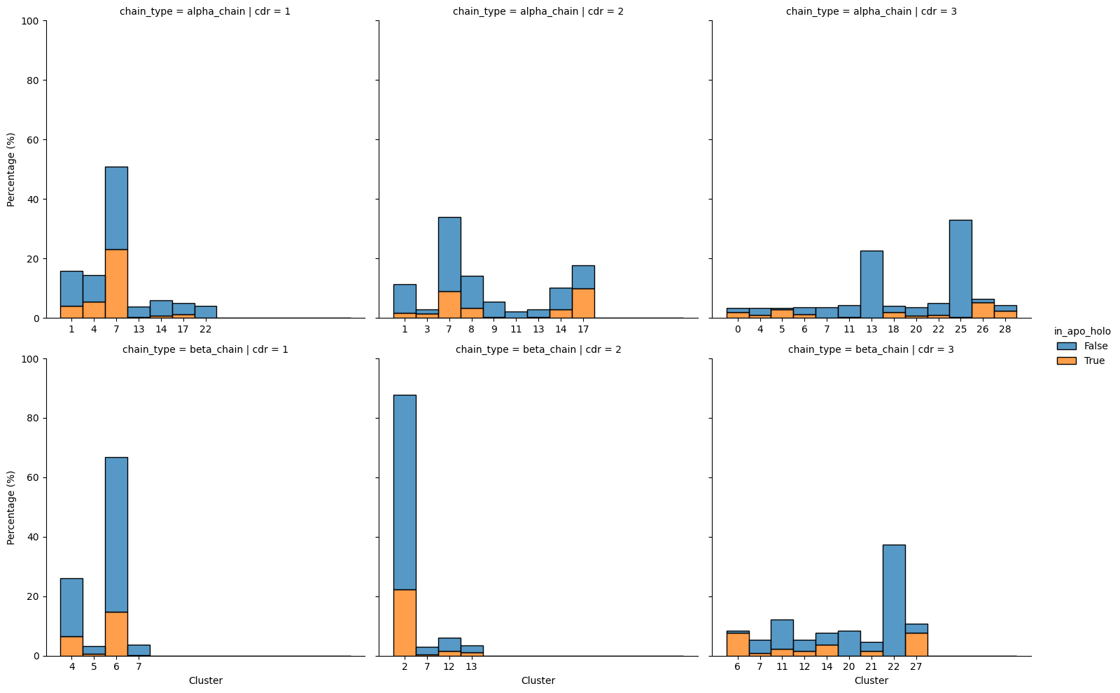
[53]:
apo_holo_coverage = (canonical_cdr_clusters.groupby(['chain_type', 'cdr', 'cluster'])
                                           .apply(lambda group: group['in_apo_holo'].any())
                                           .value_counts(normalize=True) * 100)[True]

print(f'There is {apo_holo_coverage:.2f}% coverage of canonical clusters in the apo-holo dataset.')
There is 86.96% coverage of canonical clusters in the apo-holo dataset.
Conclusion
Our analysis here shows that the conclusions drawn about TCRs from our structural analysis in this project should generalise well to other TCR:pMHC-I interactions where structure information is not currently available. The comparisons here show that the distribution of CDR lengths, amino acid compisition of CDR loops, and generally the distribution of V gene usage is comparable between the selected STCRDab structures and the background of TCRs sampled from OTS. However, it does seem that there is some over representation bias of certain V genes which may affect results. The analysis also shows that canonical CDR loop clusters are well represented in the selected analysis. We did not look at amino acid composition and other possible comparable properties from these sequences that could be done.